The Bayesian way to Statistical Significance

^{Reference to past blog: In the previous blog, I explained the way Bayesians did what Frequentists could not and solved for backward probabilities. Today I explain the Bayesian analog of a Frequentist Hypothesis Test.}

The Bayesian approach to solving the problem of statistical significance is relatively newer and has more variations to it than its Frequentist counterparts (the t-test). In particular, I have seen two Bayesian approaches to solving the same problem. Both the approaches start at the same place but differ in terms of how they call out the significance. In this blog, I will give you an outline on both the approaches and how they differ.

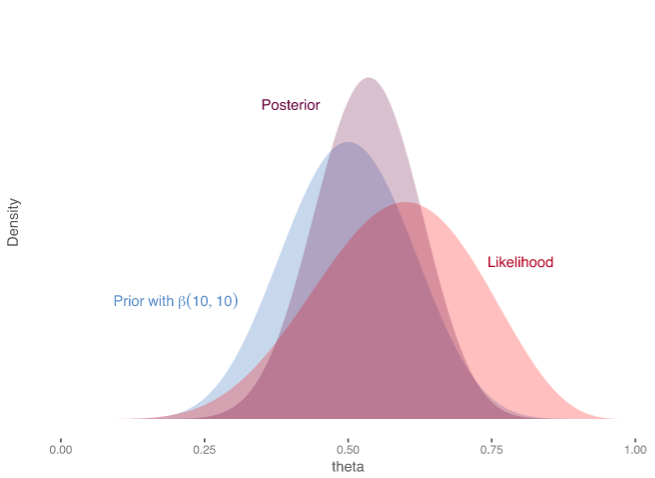
In the last blog, I explained how Bayesians invented the prior. In a usual comparison between two samples of interest, Bayesians first define a prior to represent the means of the two samples. For instance, in a Bayesian A/B test, with one control and one variation, we would usually start with two priors each representing the mean conversion rate on a particular variation. These are flat uninformative priors representing equal likelihood of all conversion rates. When the data on each of these variations arrive, we update our prior with observed data and now the posterior will be closely centred on the observed conversion rate. So for instance, we had 3 conversions out of 10 for control, the posterior for control would now be centred at 0.3 (30% conversion rate). For instance, the feature image shows a prior that is updated using the likelihood of data. The multiplication of the prior and the likelihood gives us the posterior distribution which lies somewhere in between.

This posterior also allows Bayesian to calculate the posterior on the improvement between control and variation. You need do some mathematical hocus-pocus (fairly easy) and calculate the  likelihoodness over all theoretical improvements between control variation. This distribution tells you the likelihood of the improvement (of variation compared to control) being 0% or 10% or 20% or even -20%. This is where we diverge into two separate Bayesian solutions of statistical significance that I have seen.

Bayesian Estimation Methods

One direction that you can take is that you try to estimate the most likely value of the true improvement and calculate the probability of it being greater than 0. It is possible to do this very easily as at any given point of time you have the posterior distribution over all improvements. This probability is the backward probability that tells you that looking at the data (effect) what is the chance that they come from different sources (cause)? Note how this is not the probability of a null hypothesis or the alternate hypothesis. This probability just simply tells you the probability of the improvement being greater than 0. If the probability is greater than a threshold, you can accept the decision. At VWO, we call this statistic as the Chance to Beat Control.

The Bayesian Framework allows you to answer any such question once you have the posterior. For instance you can also ask what is the chance that the improvement is greater than 2% or what is the chance that improvements are lesser than 5% and so on.

The Bayesian Estimation framework is not a framework to test hypothesis and that is why you do not see a null hypothesis or an alternate hypothesis in the Bayesian Estimation. In fact, in the Bayesian estimation framework, the null hypothesis is improvement = 0 which is just a point in the whole distribution. Essentially the probability of the null hypothesis is always 0 in the Bayesian estimation framework because even if the improvement is infitesimally small, it might still be some real valued number.

Bayesian Estimation methods define a model for the causal process and calculate the best estimated value of all parameters of the model. For instance, in the Bayesian A/B Test, the model is the two distributions representing the mean conversion rates and Bayesian Estimation helps you estimate the most likely value of these conversion rates. Bayesian Estimation does not attempt to prove or disprove a hypothesis directly.

Bayesian Hypothesis Testing

Bayesian Estimation methods are helpful in determining significance, but they are still not hypothesis testing methods. Bayesian Hypothesis Testing does everything similar to what we have done uptill the introduction. It defines the prior, calculates the posterior and then calculates the posterior over the improvement as well. However, the story ahead is a bit different.

In Bayesian Hypothesis Testing, one defines a Null Hypothesis and an Alternate Hypothesis. However, note that the null hypothesis represents only a point estimate in the posterior of improvement. Hence, for the reasoning given above, the null hypothesis in Bayesian is a point estimate (improvement - 0) and hence does not have any probability on its own. To counter this problem, the definition of a Null Hypothesis demands that you allot it a certain region around improvement = 0. This region is called the Region of Practical Equivalence (ROPE). I will touch on the topic in detail later.

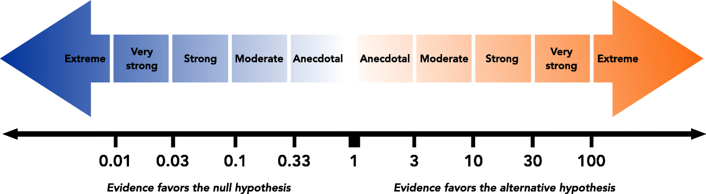
Finally, they calculate the Bayes Factor = Probability of the Null Hypothesis/Probability of the Alternate Hypothesis. The Bayes Factor comes out as a symmetric ratio between the likelihoods of the Null Hypothesis and the Alternate Hypothesis. The Bayes Factor is the proper p-value analog of Bayesian Hypothesis Testing. The interpretation of Bayes Factor is usually done as follows.

Conclusion and the way ahead

Bayesian Estimation is relatively more popular in A/B testing because most people do not understand what is the Bayes Factor. Bayesian Hypothesis Testing was independently developed in the field of Psychology and to the best of my current knowledge has not been used till date in the field of A/B Testing. The buzz is starting to float around on the Bayes Factor and it might be that in the years to come, it starts to rival the popularity of the p-value.

On the outside, both the methods of Bayesian Estimation and Bayesian Hypothesis Testing seem to be taking you to the same place by devising unique statistics for decision making. However, there are core differences in ideaology behind the two. Any hypothesis testing framework be it Bayesian or Frequentist, gives more weight to the null hypothesis which at first seems unfair. However, as you will see in the upcoming discussion it is a core fundamental of Occam's Razor.

Occam's Razor states that as long as the evidence is not starkly against, the simplest model with the fewest parameters should be preferred for any causal phenomena.

In the next discussion, we will dive deep into Frequentists vs Bayesian and savour the age-old debate.