How does a t-test work?

^{Reference to past blog: In a previous blog, I started to express my understanding of hypothesis tests. In this blog, I will take that story to the end and give you the anatomy of the basic form of a hypothesis test, the t-test.}

The road I am taking today trods slightly deeper into the forests of statistics. I will not tumble you in a lot of equations and derivations, but I will only try to explain one relationship central to all hypothesis testing. With the understanding of the right determinants, I believe the interested reader would have a facility in predicting the calculations of statistical significance.

When you ask the question of whether the observed data come from two different sources or not, essentially you talk about an underlying ground-truth common to the entire population. For instance, if you ask whether a drug is effective or not, you are asking about the efficacy of the drug on the entire population and not just the few that you test the drug upon. A core fundamental to understand is that, all experimentation is done on samples, which represent a small portion of the population. The job of hypothesis testing is to answer something about the whole population using just these samples.

Statisticians started by first modeling that depending on the size of a sample how much different can it be from the entire population. This idea gave birth to a core fundamental of statistics, The Sampling Theory.

Samples from a Population

Imagine that you want to accurately measure the average height of homo sapiens. You would ideally want a database of all individuals who have ever been born. Their mean adult height would be the actual average height of homo sapiens that you wish to measure. But real-world constraints would only let you collect a sample of this entire population and let you calculate an average on that. But the question is how off can this average be from the actual average height of human beings.

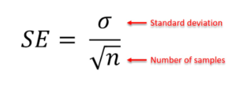
You know that this average cannot be off by a few feets because height as a variable does not have a variance of a few feet in it. And you also know that the larger the sample size the less wrong you would be. These two core factors help you decide how wrong can your sample average be as compared to your true population average. This measure is called the Standard Error (SE).

The three determinants of the statistical significance

A t-test uses the concept of a standard error to ask an interesting question, "Can the two observed sample sets come from the same population?" The following are the key ingredients you need to answer this question:

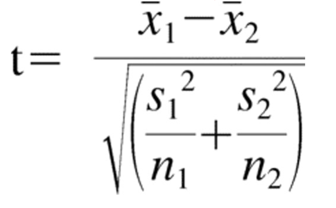
1. Effect-Size: How far off are the means of the two samples? Once you know this, you can always compare this with the standard error.
2. A combined expression of standard error: What is the combined standard error in both the samples? This expression came from some complex hocus-pocus in vector maths. The formula of this combined error can be seen in the denominator of the t-statistic where s denotes the standard deviation. The standard error incorporated both the variance and the sample size in itself.

The metric of interest was the ratio between the effect-size and the standard error (as explained earlier). This metric came to be known as the t-statistic. The t-statistic had three crucial ingredients - effect size, variances and the sample sizes.

The t-distribution

Finally, all you needed was a statistical distribution related to the t-statistic that you could use to look up how rare your calculated t-statistic actually is. This statistical distribution will give a quantitative measure to the rarity of the observed t-statistic. There is nothing so special about the t-distribution as most distributions in statistics resemble the bell curve. However, there are two things to note:

1. The t-distribution takes an input parameter called "degrees of freedom" which is always equal to (1 - sample size of the study). Hence, t-distribution is like a normal curve which can get fatter for lower degrees of freedom.
2. T-distribution is different from the normal distribution only when the degrees of freedom are below 30. Anything above 30 is like a normal distribution.

For reference, the t-distribution looks like this:

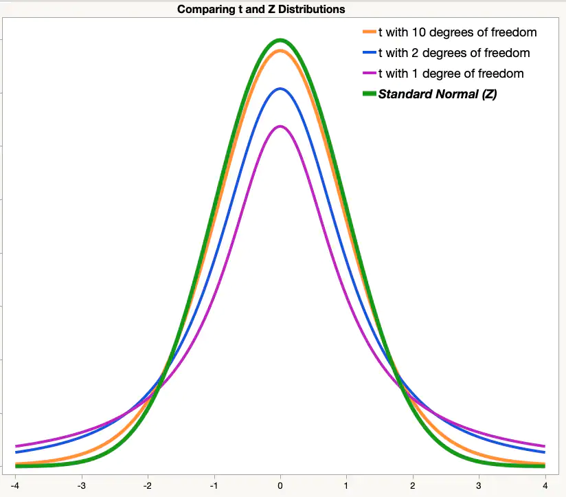
^{*Note that z-distribution is just a fancy name for normal distribution in a sampling context}.

The x-axis of the above graph places your t-statistic and the t-distribution tells you how likely is that t-statistic. The p-value is the area of the curve that cuts to the right of the calculated t-statistic.

Hence, the story is complete. The higher your standard error, the more your t-statistic move towards zero. The higher your effect size the more you swing towards the corners of the distribution reducing the p-value.

That's all that a t-test does. Sounds very complicated but once you understand what is happening you will understand that it aligns perfectly with intuition.

Numbers that vary a lot are less trustworthy to judge finer differences, things that vary less in general are more reliable for observing the finer differences. Just think of a weighing machine that keeps swinging on a range of 2 kgs. Will you trust it if tomorrow you see a 1 kg weight reduction on the machine.

The way ahead

The story until now was the story of Frequentist Hypothesis Testing which has been known and used for almost a century now. The counter-part of the Frequentist ideology is the Bayesian ideology and the dichotomy between the two is one of the most interesting debates in statistics. In the next blog, we will discuss how Bayesians broke free from the constraint of only using forward probabilities and used a smart idea of priors to finally calculate the backward probabilities to reach the straight answer to the straight question. Yet, they had their own criticisms.